 This is an open access article distributed under the terms of the Creative Commons
Attribution License (
This is an open access article distributed under the terms of the Creative Commons
Attribution License (Introduction
By using linear regression it is merely assumed rather than empirically tested that the effects of the predictor variables are linear and homogeneous1 across the distribution of the dependent variable (Koenker, 2005; Wood, 2006). This is problematic because it hinders possible practical and theoretical insights (Wilcox, 1998). Thus an important question to ask is: Are the effects studied by psychologists really linear and homogeneous?
We discuss linear regression, its linearity and effect homogeneity assumption and possible consequences if these assumptions are violated. Two techniques are suggested which can be beneficially applied when the linear regression assumptions are not met. Lastly we will second these arguments with an empirical analysis of two classical predictors of violent crime in a representative sample of German youth (N = 44.610).
Linear Regression
Linear regression and its variants like analysis of variance are arguably the most widely used statistical techniques in psychology. In linear regression, the conditional mean of the dependent variable is modeled as a linear function of some predictor variables. Linear regression is regularly used by psychologists for two tasks: (a) the prediction of y, the dependent variable, given observed x values, the predictors, and (b) to gain insight into the linear dependencies between variables. However, for the predictions to be accurate and the insights to be correct several assumptions must be met (Berry, 1993).
Linear regression has several assumptions. Among them are: Linearity, it is assumed that the relationship between the dependent variable and the predictor variables is linear, independence, the errors are independent of each other, normality, conditional on the predictors the dependent variable is normally distributed, and homoscedasticity, conditional on the predictors the variance of the dependent variable is constant. If these assumptions are fulfilled the linear regression function provides an accurate summary of the linear dependencies between variables: It is obvious that there is no non-linearity to detect, because linearity is explicitly stated in the assumptions above. Additionally, if the assumptions of normality and homoscedasticity are fulfilled it does not matter where in the distribution of the dependent variable one analyses the effect of the predictors on the dependent variable - the effect will always be the same. This means that the effect is homogeneous across the distribution of the dependent variable.
If the linear regression assumptions are, however, not met the researcher could be biased in that for example existing effects are not found and information inherent in the non-linearity and effect heterogeneity is lost (Wilcox, 1998). Figure 1 shows hypothetical examples of a linear vs. a non-linear continuous effect (upper panels) and a homogeneous vs. a heterogeneous dichotomous effect between two groups, where “heterogeneous effect” means that the effect for the mean and other measures of location differ across the distribution of the dependent variable (lower panels).
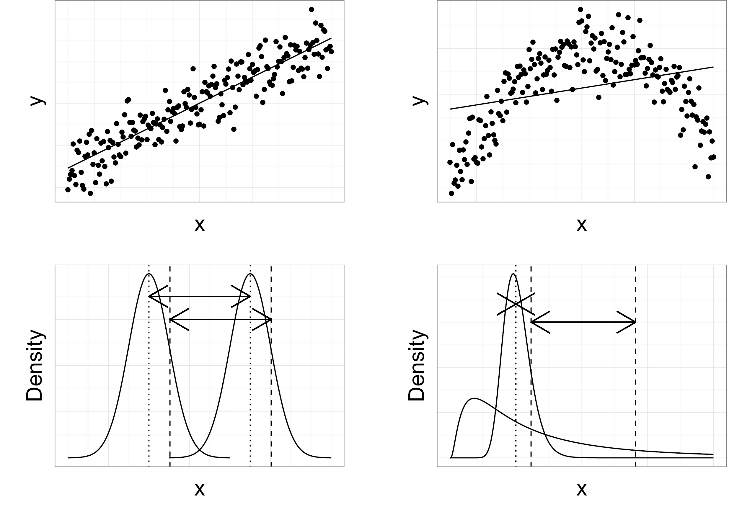
Figure 1
The linearity and effect homogeneity assumption and possible violations of these assumptions, which might bias a scientist’s reasoning. Top left: Linearity assumption is correct. Top right: Linearity assumption is violated. Bottom left: Effect homogeneity assumption is correct, i.e. the effect is the same for every part of the distribution. Bottom right: Effect homogeneity assumption is violated, i.e. the effect is not the same for every part of the distribution.
As an example, the upper panels could depict the relationship between risk-seeking and the amount of violent crime. The top left panel would thus indicate that the more risk a person seeks, the larger the number of violent incidents is. The top right panel on the other hand shows an inverted-u relationship: The highest amount of violent crime would thus result from a moderate risk-seeking value (e.g. because high risk-seekers tend to participate in a lot of sport activities, which may promote health behavior in general). The lower panels contain two distribution curves each, which might represent the amount of violent crime for people with and without drug dependence: In the bottom left panel one can see a shift effect, i.e. the amount of violent crime is higher for individuals with drug dependence and this applies to every part of the dependent variable distribution (as indicated by the two arrows, which are of the same length). However, this holds not true for the bottom right panel, which depicts a heterogeneous effect. Here drug dependence increases the amount of violent crime for the highly violent individuals (upper part of the distribution) but diminishes it for slightly violent criminals (lower part of the distribution). Thus, though there is no effect for the mean (indicated by the “X”), there is a large effect for, for example, the 85% quantile (indicated by the arrow).
It is clear from Figure 1 that undetected non-linearity or effect heterogeneity can severely bias a scientist’s reasoning. In both the top and bottom panels by using linear regression one could conclude that the predictor has no effect on the dependent variable: For the top right panel the predictor will be insignificant and the model will have an overall low R2 because the regression line doesn’t describe the data well. In the bottom right panel there is simply no effect for the mean to detect (dotted lines) because the means of the two groups are identical. There is however a rather large effect for the 85% quantile (dashed lines), which cannot be discovered by the usual statistical techniques like linear regression. Thus in the case of the bottom right panel the researcher might falsely conclude there to be no effect when in reality the effect might be rather large for some participants like those corresponding to the 85% quantile. Additionally, besides not finding an existing effect, the researcher might also be biased in that an effect’s magnitude is overestimated, underestimated or a non-existing effect is erroneously assumed to exist.
Furthermore a violation of these assumptions might be the norm rather than the exception in original as well as meta-analytical research (Kliem, Beller, & Kröger, 2012; Micceri, 1989). This also fits with our every-day observations that social phenomena exhibit a high variability across individuals and contexts. Thus there is a need to go beyond the usual linear regression analyses in psychological research.
Alternatives to Linear Regression
Generalized additive models. The generalized additive model (GAM) is a statistical technique which combines traditional linear models with additive models (Hastie & Tibshirani, 1990; for a recent introduction see e.g. Wood, 2006). It differs from ordinary linear regression in that the linear terms are replaced by non-parametric smooth functions of the predictor variables to give
A “sum-to-zero” constraint on each fj ensures identifiability. These non-parametric functions automatically adapt to non-linearities in the data. Furthermore, because the linear effects are nested in the GAM specification one can also statistically test whether the effects are significantly non-linear. Controlling for over-fitting via cross-validation no a priori assumptions regarding the form of non-linearity must be made. Thus GAMs can answer questions regarding the possible non-linear effects of predictor variables: For example, is there a certain amount of alcohol consumption which must be breached in order for alcohol consumption to become an increasingly important risk factor for violent behavior?
Quantile Regression. Quantile regression (Koenker & Bassett, 1978; for a recent introduction see e.g. Koenker, 2005) is a statistical technique, which enables the researcher to not only model the conditional mean but also the median and other quantiles of the dependent variable. Thus via quantile regression two questions can be answered: Do the predictors have an effect across the distribution of the dependent variable? And if so, do these effects differ across the distribution of the dependent variable? For example, quantile regression might be beneficially applied when one is not most interested in the mean but in extremes such as the 90%-quantile. Educational psychologists might, for example, be interested in the heterogeneous effects of an after-school achievement program, which inherently should work most for extreme cases such as highly disadvantaged children.
Benefits. The use of GAMs and quantile regression has many advantages: For the practitioner it is important to know whether the effect is non-linear or varies with the distribution of the dependent variable. Such knowledge could help social workers to adapt their intervention strategies on the concrete person and context rather than relying on a one-size-fits-all “mean” effect. Additionally it is theoretically important to establish whether an effect is non-linear or varies across the distribution of the dependent variable. This finding might, for example, uncover the generalizability of effects.
Example: Do two Classical Predictors for Violent Crime Exhibit Non-Linear and Heterogeneous Effects?
In the following the possible practical and theoretical benefits of going beyond the usual linear regression analysis are exemplified. We utilize GAM and quantile regression separately for ease of interpretation although these two techniques might also be combined (Koenker, 2011). The dataset consists of a representative survey of youths in the 9th class in Germany from 2007 and 2008 (N = 44.610). The survey was conducted by the Criminological Research Institute of Lower Saxony. The participants had to indicate how much incidents of actual bodily harm, grievous bodily harm, robbery, extortions and sexual violence they caused in the last 12 months; the sum of these incidents is used as the dependent variable.
Two of the most important and most studied predictors of violent crime are risk-seeking and criminal peer networks. Regarding risk-seeking Gottfredson and Hirschi’s (1990) general theory of crime posits that low self-control is the main driving factor behind crime. Risk-seeking is one major aspect of low self-control meaning that individuals with high risk-seeking tend to favor the immediate gain of the moment instead of foregoing the currently available pleasure for long-term benefits. Risk seeking was measured via four four-point Likert items of a questionnaire. The predictor risk-seeking was operationalized as the mean of this scale. Criminal peer network denotes the number of criminal friends. For example, Rabold and Baier (2011) recently showed that friendship networks play a major role in explaining ethnic differences in crime rates. Participants were asked to indicate how much criminal friends they had regarding two different aspects of violent crime on two six-point Likert scales. The mean was taken as the second predictor. Missing values were imputed via the missForest algorithm (Stekhoven & Bühlmann, 2012). Prior to the analyses the covariates have been standardized. All analyses were conducted in R (R Core Team, 2012): The mgcv package was used for the GAMs analysis (see e.g. Wood, 2006); for the quantile regression analysis the quantreg package was used (see e.g. Koenker, 2005).
Results and Discussion. The linear regression analysis replicates risk-seeking and the number of criminal friends as significant predictors for the amount of violent crime; risk-seeking: b = 0.43, se = 0.02, p < .001; criminal peer network: b = 1.34, se = 0.02, p < .001.
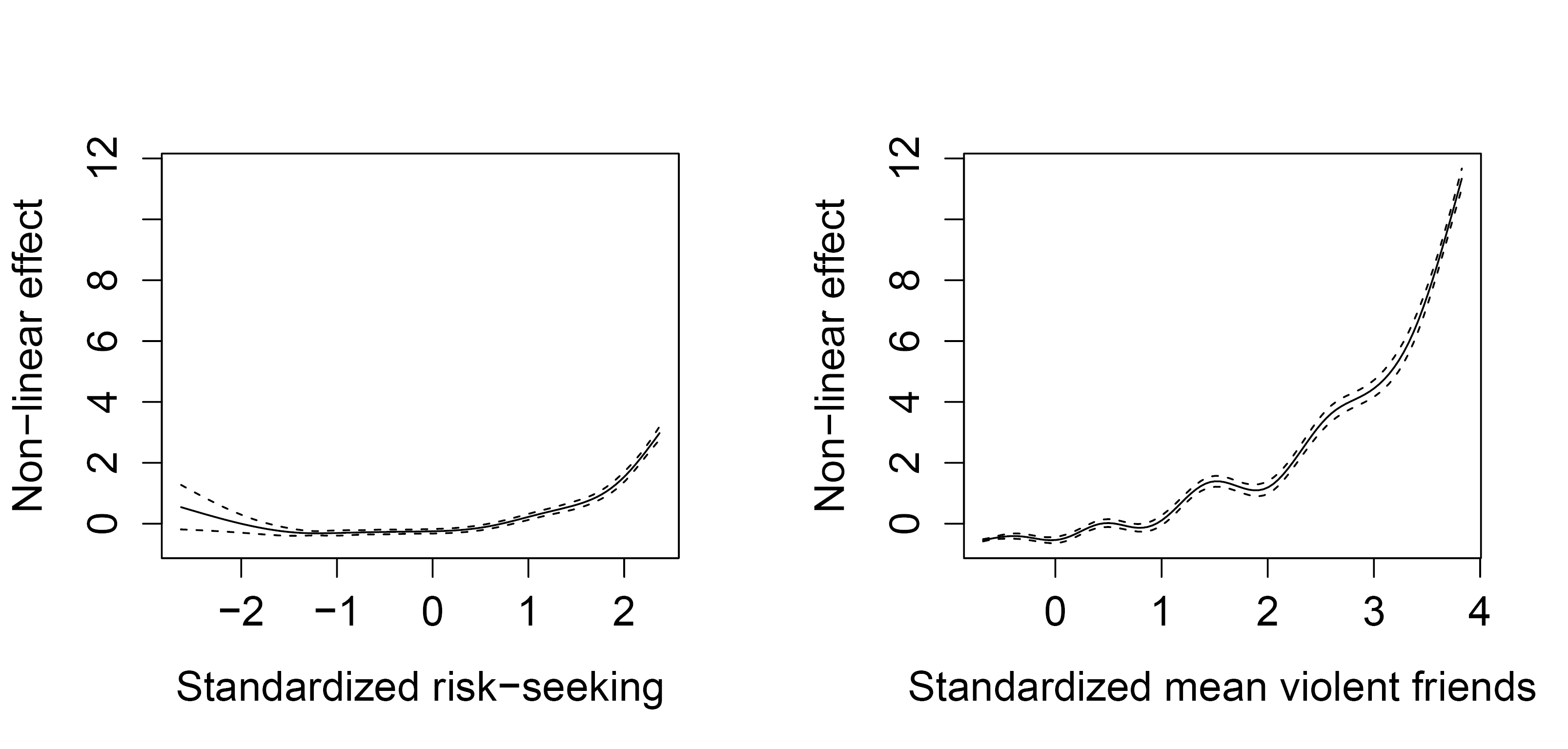
Figure 2
Non-linear effects of risk-seeking and criminal peer network.
The GAM analysis indicates both coefficients to be significant predictors of violent incidents, both p-values < .001, seconding the linear regression results. Testing for non-linearity the GAM analysis additionally shows that these coefficients are significantly non-linear, F(15, 44592) = 218.07, p < .001. Figure 2 displays the nonlinear regression coefficients of the predictors on the scale of the linear predictor (x-axis). From the figure it can, for example, be seen that after about half a standard deviation above the mean (0.5) the effect of risk-seeking increases steadily. This corresponds to a value of about > 2.5 in our risk-seeking scale. The effect of criminal peer networks on the other hand increases in an exponential fashion from the beginning on (the dips most possibly occur here because two Likert scales were used to measure the number of violent friends).
Analyzing the same dataset via quantile regression yields the following complementary results, which are summarized in Table 1. The coefficients are highly heterogeneous across the upper part of the distribution of the dependent variable, F(8, 223042) = 88.59, p < .001 (see also Table 1). In general, the coefficients increase with higher quantiles. This means the more violent crimes are done, the more influence is exhibited by the predictors. Or, equivalently, the predictors are most meaningful in modeling highly criminal individuals but less so in slight violent criminals.
Table 1
Quantile Regression Results for the 0.85, 0.9, 0.95, 0.99 and 0.999 Quantile
| Predictors | 0.850 | 0.900 | 0.950 | 0.990 | 0.999 |
|---|---|---|---|---|---|
| Risk-seeking | 0.00 | 0.00 | 0.15* | 1.92* | 6.16* |
| (0.06) | (0.07) | (0.05) | (0.79) | (1.25) | |
| Criminal friends | 1.85* | 2.96* | 5.49* | 12.64* | 15.85* |
| (0.14) | (0.15) | (0.15) | (0.83) | (1.64) |
Note. Standard errors are depicted in parentheses.
*p < .05.
Both analyses are practical and theoretical important. For example, imagine a social worker, who knows which factors are truly risk-factors for his specific clients: Based on our GAMs analysis this might for example be a predominant criminal peer network or an especially high amount of risk-seeking. Additionally by modeling different quantiles it has been shown that risk-seeking is not a general risk factor for crime (as suggested by proponents of the general theory of crime): Contrary, only the 5% most violent offenders are slightly affected by risk-seeking in their crime rate. Thus important practical and theoretical implications can be discovered when going beyond the usual linear regression analysis.
Conclusion
It was shown that the usual linear regression assumptions might bias a scientist’s reasoning if these assumptions are not met. Furthermore we introduced and exemplified two complementary approaches, GAMs and quantile regression. Both techniques are able to detect interesting patterns in the data, which would have typically been obscured by linear regression. Thus both techniques should be used more often in psychological research. So, which effects of psychology are non-linear and heterogeneous? It is difficult to speculate on this, but for the advancement of psychological science we think it is of utmost importance to find out.